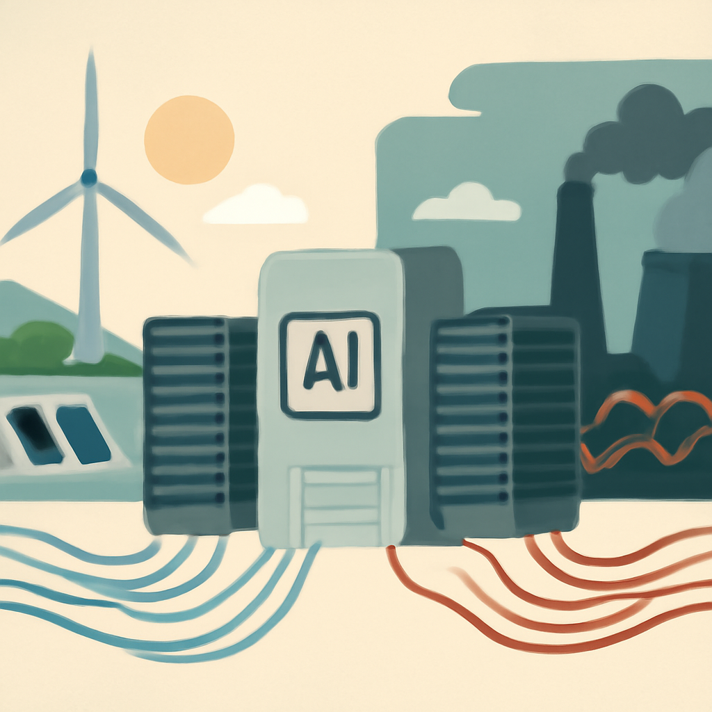
Short answer: yes, a modeled AI request can come out much higher in one place than another—but 8.5× is not a universal fact about every prompt.
The headline number comes from a calculator-driven comparison, not from a universal measurement of all AI traffic. In the example described by Berget AI, an otherwise similar inference request can have very different estimated CO₂ emissions depending on where it runs, because the electricity grid, cooling overhead, hardware efficiency, and modeling assumptions all change the result. That makes the comparison useful for planning, but not a substitute for provider-audited emissions data or a promise that every request will scale by the same factor.
The most important takeaway is practical: location can matter a lot, but the estimate is only as good as the inputs. If you use it wisely, it can help teams choose cleaner regions, compare deployment options, and identify avoidable waste. If you use it as a precise label for a single request, you will overstate what the number proves.
What the 8.5× headline does—and does not—prove
The Berget AI press release frames the result as a per-request comparison, and the open-source calculator shows how the estimate is built. But the ratio is modelled under specific assumptions, not directly observed for every AI inference request in the wild. That matters because two “similar” requests may still differ in token count, batch size, model variant, hardware class, cooling design, and the local grid at the moment they run.
The repository’s example is especially useful because it exposes the moving parts. For a Gemma 4 31B example, the calculator shows roughly 43.4 mg CO₂ in Sweden versus 311.4 mg for the U.S. average, which is about 7.2× when you include the modeled total excluding training. It also separates out an operational-only comparison of about 56.7×, with the embodied hardware component changing the final ratio. Those are not contradictions—they are reminders that “the number” depends on what is counted.
So the 8.5× claim is best read as a configured comparison that illustrates possible variation, not a universal benchmark for all AI requests, all regions, or all providers.
What changes the estimate?
Here is the compact version of the main drivers behind a per-request CO₂ estimate.
- Grid carbon intensity: cleaner electricity lowers operational emissions; dirtier electricity raises them.
- PUE and cooling: data centers with higher power overhead emit more per unit of useful computing.
- Hardware utilization: poorly utilized servers spread infrastructure emissions over fewer useful requests.
- Model size and architecture: larger models usually need more compute and memory, increasing energy per request.
- Response length: longer outputs mean more tokens and more inference work.
- Embodied hardware: servers carry manufacturing emissions that can be allocated across their lifetime usage.
- Training emissions: if included or amortized, they can dwarf inference for some models; the calculator excludes them by default.
- Workload timing and region: running at cleaner times or in cleaner places can materially change the estimate.
In other words, a request is not “just a request.” It sits inside a system: a model, a server fleet, a cooling design, a grid mix, and a set of accounting rules.
A simple comparison table
The table below shows how the estimate can move when assumptions change. The values are illustrative of the calculator’s modeled comparison, not audited provider emissions.
- Sweden example: lower modeled CO₂ because the grid is cleaner and the operational footprint is lower.
- U.S. average example: higher modeled CO₂ because the average grid is more carbon-intensive.
- Operational-only view: can show a much larger regional gap because it excludes embodied hardware.
- Total excluding training: blends operational emissions with embodied hardware and is often the most intuitive request-level view.
- Including training amortization: can change the picture significantly, but should be handled carefully because training is a separate lifecycle component.
Why the calculator excludes training by default
Inference emissions and training emissions answer different questions. Inference is the carbon cost of serving a user request. Training is the carbon cost of building the model in the first place. Combining them into one request-level number can be misleading unless you are explicit about how training is allocated across future usage.
That is why the calculator excludes amortized training by default: the tool is trying to estimate the emissions of a specific request, not to re-price the entire model development lifecycle every time someone asks a question. This is a sensible default for operational decision-making, but it also means the result is incomplete if your reporting goal is full lifecycle accounting.
The IEA’s Energy and AI executive summary is useful context here: AI-related electricity demand is a systems issue, not a single-metric issue. Any serious carbon estimate needs to distinguish between electricity use, infrastructure overhead, and lifecycle effects rather than collapsing everything into one neat number.
Why embodied hardware matters, even when it is uncertain
Servers do not appear out of thin air. They must be manufactured, transported, operated, and eventually replaced. The calculator attempts to account for embodied hardware, but the repository itself notes uncertainty in that component—roughly ±30–50%—and asks for real-world validation. That is a healthy warning, not a flaw to hide.
Embodied emissions matter more when utilization is low. If a cluster is underused, a larger share of the manufacturing footprint is effectively assigned to each request. If utilization is high, the same embodied footprint is spread across more compute. That is one reason two deployments with the same model and grid can still have different per-request emissions.
What the open-source methodology lets you inspect
The value of the GitHub repository is not just the result; it is the transparency. You can inspect the assumptions, see how the calculator handles inputs, and understand which pieces are modeled versus directly measured. That is a major improvement over opaque carbon scores that cannot be checked or adapted.
The Green Software Foundation’s SCI-AI specification is relevant for the same reason. It pushes the field toward a structured way to think about software carbon intensity, including AI workloads, so teams can compare implementations more consistently. Even then, specification is not the same as audit: standards help measurement, but they do not eliminate uncertainty.
A safer way to compare two deployment regions
If the goal is to compare two regions responsibly, the safest workflow is straightforward. First, hold the model, hardware, token count, and other workload assumptions constant so you are not mixing apples and oranges. Then compare grid intensity and PUE separately, because those two inputs capture the biggest operational differences between locations. After that, split operational emissions from embodied emissions instead of folding them into one opaque total. Once the structure is clear, run sensitivity ranges so you can see how much the answer moves when the grid, utilization, or cooling assumptions change. Finally, validate the modeled result against production telemetry where possible, because the best comparison is one that survives contact with actual workload data.
This approach does not remove uncertainty, but it makes the uncertainty visible. It also helps avoid a common mistake: treating a region comparison as if it were a fixed property of geography rather than the output of a specific accounting model. In practice, the cleanest comparison is the one that keeps the number of moving parts small enough to interpret and large enough to be realistic.
Eight checks before you trust the number
- 1. Ask what is being compared: one request, one token, one session, or one million requests? The denominator changes everything.
- 2. Confirm the model and response length: a bigger model or longer output can materially increase emissions.
- 3. Check the region and grid data: the carbon intensity of electricity is often the largest regional driver.
- 4. Look for PUE or cooling assumptions: infrastructure overhead can move the result even when compute is unchanged.
- 5. Separate operational from embodied emissions: do not mix them without stating it clearly.
- 6. See whether training is excluded or amortized: inference-only and lifecycle views answer different questions.
- 7. Review uncertainty bounds: embodied estimates in the repository are explicitly uncertain, so precision should be treated as approximate.
- 8. Validate against real workloads: use the calculator for planning, then compare with production telemetry where possible.
How developers can act on the estimate
Carbon-aware deployment does not mean guessing the greenest story. It means making workload decisions with enough discipline to avoid false precision. For engineering and cloud teams, that can include choosing cleaner regions when latency and compliance allow, shifting non-urgent jobs to cleaner times, reducing response length, right-sizing models, improving utilization, and avoiding idle capacity.
Electricity Maps has documented a similar principle in its case study on Google data centers: shifting computations to cleaner times and locations can lower emissions without changing the core service. That does not mean every workload can move freely, but it does show that operational scheduling is part of carbon strategy, not an afterthought.
The safest posture is to treat carbon estimates as decision support. They are best used to compare options, identify hotspots, and prioritize improvements—not to claim a precise gram-level truth for a single AI prompt.
Bottom line
Yes, the same AI request can be estimated at dramatically different CO₂ levels in different places. But the 8.5× figure is a modeled comparison, not a universal law. The real lesson is that grid intensity, cooling overhead, utilization, model size, response length, embodied hardware, and training-accounting choices all change the answer. If you understand those levers, you can make better deployment decisions without pretending the estimate is exact.
Sources
- Berget AI press release: https://berget.ai/en/blog/per-request-co2-press-release
- Open-source calculator and methodology: https://github.com/berget-ai/co2-calculator
- Electricity Maps case study: https://www.electricitymaps.com/resources/case-studies/google-data-centers-shift-their-computations-to-cleaner-times-and-locations
- IEA Energy and AI executive summary: https://www.iea.org/reports/energy-and-ai/executive-summary
- Green Software Foundation SCI-AI specification: https://github.com/Green-Software-Foundation/sci-ai